Copyright (c) 2026 Jan Philipp Thiele and Andrea Morini SPDX-License-Identifier MIT
201: Using StatFEM on a 2D Plate with a hole
In this example the statistical finite element method (StatFEM) is used to calculate a Bayesian posterior of a sampled finite element solution (prior) based on given data at sensor locations.
The underlying setup is a 2-dimensional plate with a hole, with a mesh given in Example201_mesh.msh. The figure shows the mesh as well as the sensor locations 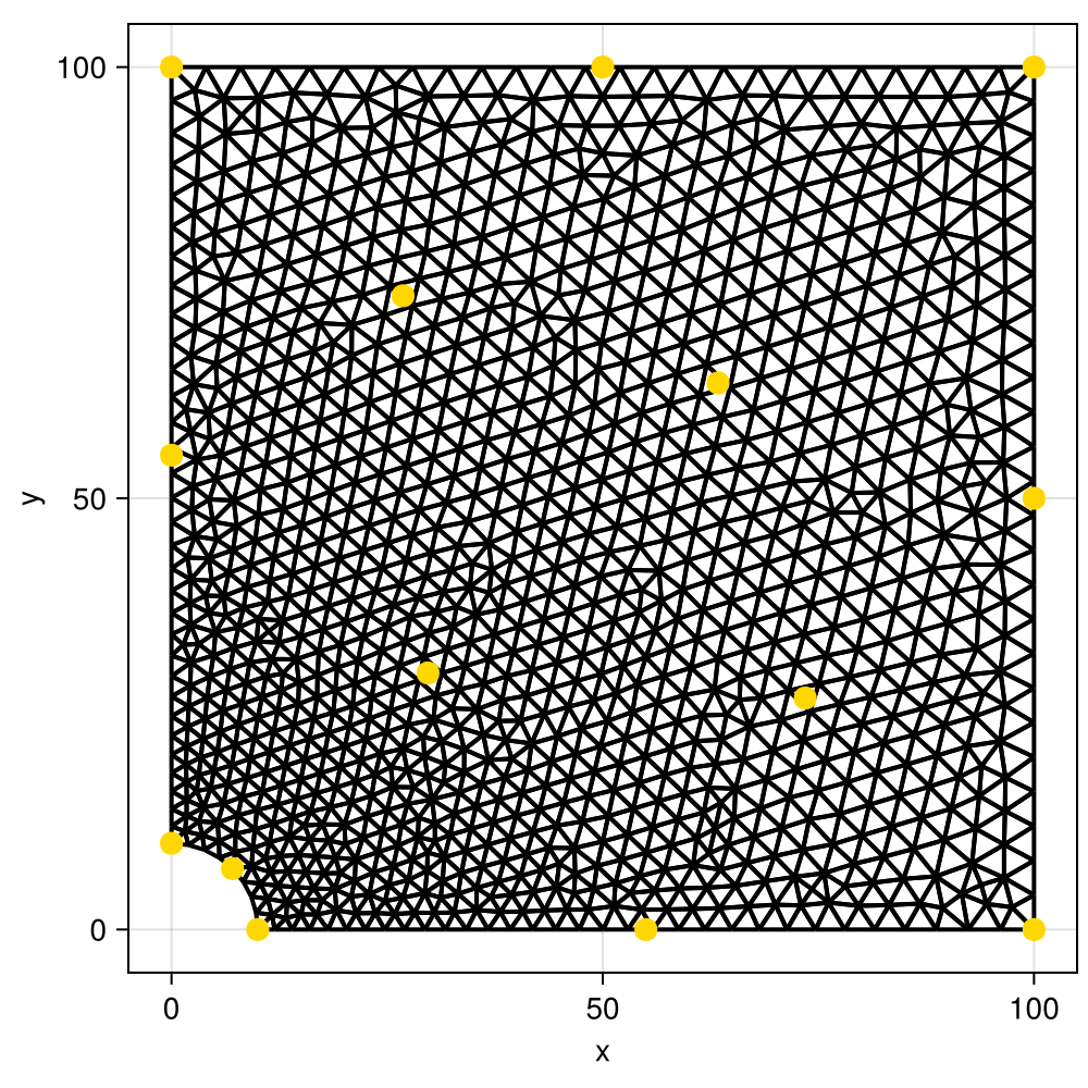
Since the mesh only contains a quarter of a full plate, we apply symmetry conditions, e.g. zero normal displacements, on the left and bottom boundary. A traction force is applied to the right boundary (boundary id 1) and the top is a free boundary.
Instead of experimental data we have generated synsthetic measurements by by solving the problem with a Mooney-Rivlin model with the mean traction $\mu_F=0.5$. The resulting full field solution is first mapped to the sensor locations and then perturbed by a Gaussian noise sample for each of the sensor points. This data is available in Example201_measurements.csv
For the StatFEM assimilation we start like in Example101 by calculating a PCE surrogate for the sampled displacements. For the sampling we solve the problem with a linear elastic material with parameters corresponding to the Mooney-Rivlin parameters. With the PCE surrogate, the measurement data and projection from the sensor locations we use StatFEM to calculate the posterior mean and covariance. For a better visual comparison we plot the prior and posterior displacements and their confidence intervals (CI) along bottom boundary. 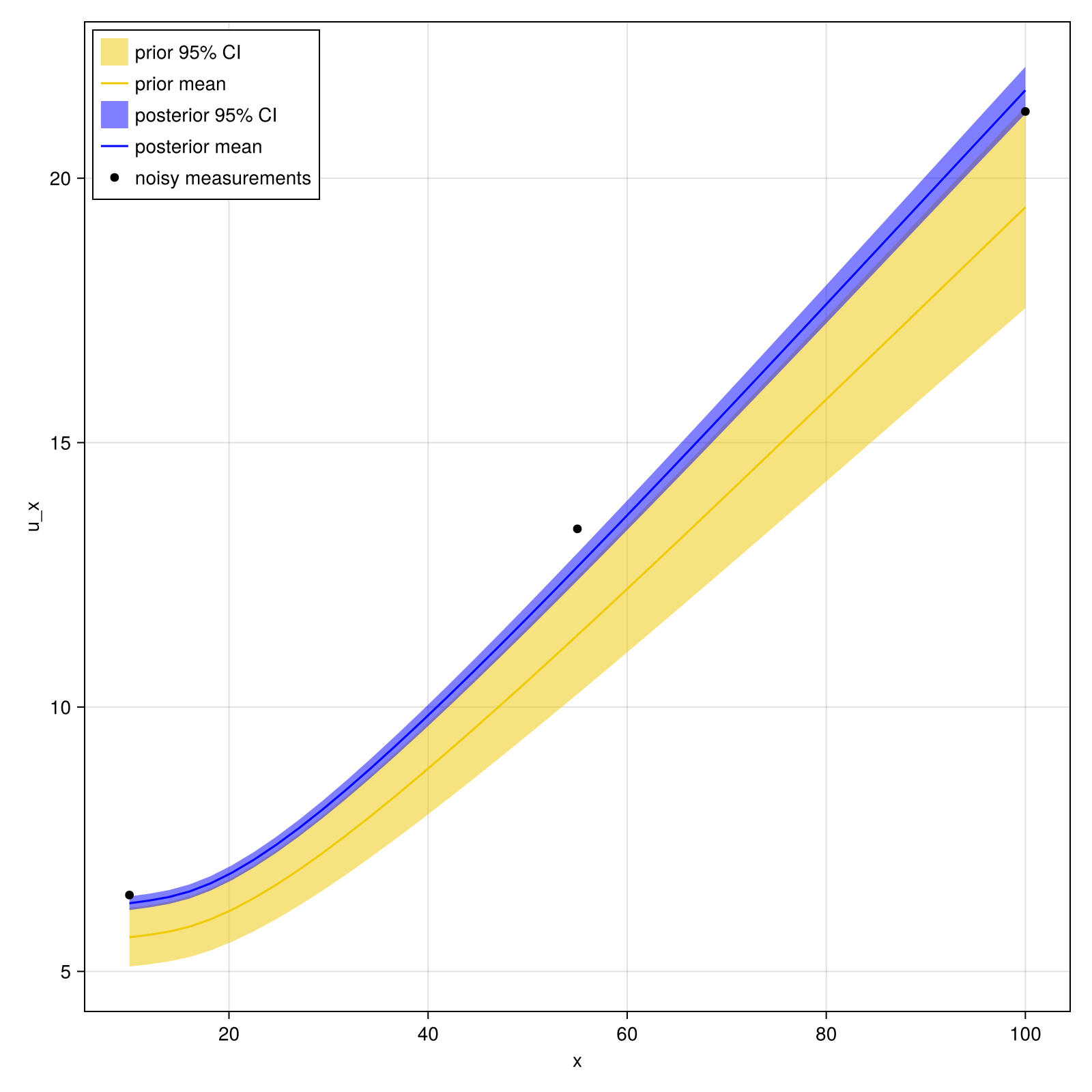
If you want to regenerate the synthetic measurement data you will need a server that is capable of solving the problem with the Mooney Rivlin model. The generation is done through the generate_synthetic_data function, where you can pass the server_url matching your server. The data in the repository was generated with the Ferrit.jl-based server.
module Example201_StatFEM_PlateWithHole

using StatFEMEUCLID
using Random
using Distributions
using UMBridge
using CairoMakie
using Gmsh
using ExtendableGrids
using GridVisualize
using CSV, DataFrames
using PolyChaos
using LinearAlgebra: diag
If the forward model does not provide a projection (see below) we can use the StatFEMEUCLID extension enabled by loading ExtendableFEMBase
using ExtendableFEMBaseWith server_url you can point to a different UMBridge server implementing the model the default is what is provided by the Ferrite.jl-based implementation here. An alternative is provided by the Kratos-based implementation here with server_url="http://localhost:4242. Note that the Kratos implementation only provides the linear elasticity model, so it can not be used for the data generation.
function main(;
        μ_F = 0.5,
        σ_F = 2.5e-2,
        n_PCE = 30,
        E = 2.7,
        ν = 0.35,
        σ_sensor = 0.5,
        server_url = "http://localhost:4232",
    )

    rng = MersenneTwister(2530)  #fixed seed for comparability between runs
As in Example101 we start by defining UMBridge HTML models for querying the forward model
    model_name = "HolePlate2D"
    fem_model = UMBridge.HTTPModel(model_name * ".FEM", server_url)
Additionally, we need the projection from degrees of freedom to the sensor locations. The ordering should follow the ordering given by the mesh file, otherwise the plotting will produce wrong results. The consistent option has the server provide this mapping.
projection_model = UMBridge.HTTPModel(model_name * ".projection", server_url)For calculating the projection on the client side we have to provide the grid but we also need it for plotting, so we load it early
grid = ExtendableGrids.simplexgrid_from_gmsh("Example201_mesh.msh", Tc = Float64, Ti = Int64)Since some of our example servers can solve for more than one material model we now need to specify this in a configuration. However, if the server only solves linear elasticity this can and would be ignored by default.
    LE_material_config = Dict{String, Any}(
        "material" => "LinElastic"
    )
In general, we want to be able to change other parameters, in the case the material parameters. Therefore, these are passed as additional arguments through UMBridge, such that the server should expect an input vector [[F],[\nu,E]] in case of linear elasticity, or in general [[F],[extra_params]]. The additional parameters are passed with the optional extra_params keyword argument.
    ux_prior_sample = sample_FEM(
        fem_model,
        n_PCE,
        sample_distribution = Normal(μ_F, σ_F),
        rng = rng,
        config = LE_material_config,
        extra_params = [ν, E]
    )
For statFEM we need three components, a PCE surrogate, measurement data and a projection matrix H from our solution space (dofs) to the locations of the sensors where the measurements were taken.
1 PCE surrogate, see Example101
ux_pce_surrogate = PolyChaosExpansion(ux_prior_sample, polynomials = GaussOrthoPoly(4))2 Sensor points from file + projection matrix
sensor_set = CSV.read("Example201_sensors.csv", EqualSensorSet{Float64}, σ_sensor)If your forward model provides the projection you build the matrix with the following commands
n_dofs = UMBridge.model_output_sizes(fem_model)[1]
calculate_projection_matrix(sensor_set, projection_model, n_dofs)
Otherwise the extension provides (needs using ExtendableFEMBase)
calculate_projection_matrix(sensor_set, grid)3 Read in (synthetic) measurements
    dataframe_measurements = CSV.read("Example201_measurements.csv", DataFrame)
    measurements = [Vector{Float64}(row) for row in eachrow(dataframe_measurements)]

    ux_measurements = zeros(length(measurements))
    for i in eachindex(measurements)
        ux_measurements[i] = measurements[i][1]
    end
With all components in place, we can now calculate the posterior statistics, i.e. the vector of nodal mean values and covariance matrix.
    ux_posterior, C_ux_posterior = posterior_statistics(sensor_set, ux_measurements, ux_pce_surrogate)
    σ_ux_posterior = sqrt.(diag(C_ux_posterior))
Finally, we want to plot the sensor locations as well as the prior and posterior along the bottom boundary Plot of sensor points and mesh
    sensorvis = plot_sensors(grid, sensor_set.locations)

    displt = plot_displacements_along_bottom_boundary(grid, sensor_set.locations, measurements, ux_pce_surrogate, ux_posterior, σ_ux_posterior)

    return sensorvis, displt
end
This function plots the measurements as well as prior and posterior displacements with confidence intervals on the line along the bottom boundary of the domain.
function plot_displacements_along_bottom_boundary(grid, sensor_points, measurements, pce_surrogate, μ_posterior, σ_posterior)
    f = Figure(size = (800, 800))
    ax = Axis(f[1, 1], xlabel = "x", ylabel = "u_x")
Get the subgrid corresponding to the bottom boundary (boundary id=3)
    sub = subgrid(grid, [3], boundary = true)
    bottom_x_grid = Float64.(sub[Coordinates])[1, :]
Need to specify full name here as compute_statistics is also part of Statistics
μ_PCE, σ_PCE = StatFEMEUCLID.PCE.compute_statistics(pce_surrogate)Extract the values at the boundary DoFs
    bottom_μ_PCE = μ_PCE[sub[NodeParents]]
    bottom_σ_PCE = σ_PCE[sub[NodeParents]]
    bottom_μ_post = μ_posterior[sub[NodeParents]]
    bottom_σ_post = σ_posterior[sub[NodeParents]]
Calculate upper and lower percentiles for the PCE prior and posterior
    confidence_factor_95p = 1.96
    lower_percentile_PCE = bottom_μ_PCE - confidence_factor_95p * bottom_σ_PCE
    upper_percentile_PCE = bottom_μ_PCE + confidence_factor_95p * bottom_σ_PCE
    lower_percentile_post = bottom_μ_post - confidence_factor_95p * bottom_σ_post
    upper_percentile_post = bottom_μ_post + confidence_factor_95p * bottom_σ_post
Find all sensor points which lie on the bottom boundary
    bottom_ids = findall(x -> x[2] < 1.0e-12, sensor_points)

    bottom_ux = zeros(length(bottom_ids))
    bottom_x_sen = zeros(length(bottom_ids))
    for i in eachindex(bottom_ids)
        bottom_x_sen[i] = sensor_points[bottom_ids[i]][1]
        bottom_ux[i] = measurements[bottom_ids[i]][1]
    end
Finally, plot both prior and posterior with confidence bands
    band!(f[1, 1], bottom_x_grid, lower_percentile_PCE, upper_percentile_PCE; label = "prior 95% CI", color = (:gold2, 0.5))
    lines!(f[1, 1], bottom_x_grid, bottom_μ_PCE; label = "prior mean", color = :gold2)
    band!(f[1, 1], bottom_x_grid, lower_percentile_post, upper_percentile_post; label = "posterior 95% CI", color = (:blue, 0.5))
    lines!(f[1, 1], bottom_x_grid, bottom_μ_post; label = "posterior mean", color = :blue)
as well as the measurement data
    scatter!(f[1, 1], bottom_x_sen, bottom_ux; label = "noisy measurements", color = :black)
    axislegend(ax, position = :lt)

    return f
end
Plot the underlying grid as well as the sensor points
function plot_sensors(grid, sensor_points::Vector{Vector{Float64}})

    sensorvis = GridVisualizer(; Plotter = CairoMakie)

    gridplot!(sensorvis, grid, show_colorbar = false)
    x = zeros(length(sensor_points))
    y = zeros(length(sensor_points))
    for i in eachindex(sensor_points)
        x[i] = sensor_points[i][1]
        y[i] = sensor_points[i][2]
    end
    customplot!(sensorvis) do ax
        CairoMakie.scatter!(ax, x, y, color = :gold, markersize = 15)
    end
    return sensorvis
end
This function generates the synthetic data based on a Mooney-Rivlin model. Note that the forward model has to be able to solve with this material model to regenerate the data. The data in the repository has been generated using the default, i.e. the Ferrite.jl-based implementation here
function generate_synthetic_data(;
        F = 0.5,
        σ_sensor = 0.5,
        server_url = "http://localhost:4232"
    )
Note that we also need the projection model here since we want to map the FEM solution to the given sensor points.
    model_name = "HolePlate2D"
    fem_model = UMBridge.HTTPModel(model_name * ".FEM", server_url)
    projection_model = UMBridge.HTTPModel(model_name * ".projection", server_url)

    A_10 = 0.3
    A_01 = 0.2
    B_1 = 1.5

    κ = [A_10, A_01, B_1]
We want to solve with the smallest Mooney-Rivlin model with a total of three parameters
    MR_material_config = Dict{String, Any}(
        "material" => "MooneyRivlin",
        "n_MR" => 1,
        "n_VOL" => 1
    )
    n_dofs = UMBridge.model_output_sizes(fem_model)[1]
Since we solve with the exact mean traction force, we don't have to sample and can directly evaluate the forward model once.
    u_truth = evaluate_fem_model(
        fem_model, F, solution_index = :, config = MR_material_config, extra_params = κ
    )
Then, we read in the sensor locations and obtain the projection matrix
    sensor_set = CSV.read("Example201_sensors.csv", EqualSensorSet{Float64}, σ_sensor)
    n_sen = size(sensor_set)
    calculate_projection_matrix(sensor_set, projection_model, n_dofs)
and project the solution onto the sensor points
u_measured = project(sensor_set, u_truth)Finally, we apply a Gaussian noise to the projected measurements
apply_noise!(sensor_set, reshape(u_measured, (n_sen, 2)); rng = MersenneTwister(2530))before writing the result to file.
    dataframe_measurements = DataFrame(u_x = u_measured[1:n_sen], u_y = u_measured[(n_sen + 1):(2 * n_sen)])
    return CSV.write("Example201_measurements.csv", dataframe_measurements)
end


#The following functions override the default behaviour of GridVisualizeTools
#to remove coloring of cells and boundaries from the sensor plot.
using Colors
import GridVisualizeTools: region_cmap, bregion_cmap
function region_cmap(n)
    return fill(RGB(1.0, 1.0, 1.0), n)
end

function bregion_cmap(n)
    return fill(RGBA(0.0, 0.0, 0.0, 0.0), n)
end

end
This page was generated using Literate.jl.