Copyright (c) 2025-2026 Jan Philipp Thiele SPDX-License-Identifier: MIT

101 : Sampling of a 1D Bar under tension

(source code)

This setup is based on the example described in section 2.3^[Narouie23].

It compares classical Monte Carlo sampling, with $n_{MC} = 1000$, to a surrogate model based on polynomial chaos expansion (PCE), with $n_{PCE} = 50$.

Instead of having a 'hard-wired' FEM package solve the underlying problem, we use UMBridge to link to a specific implementation. This black box should provide a model named Bar1D.FEM with an evaluate function solving the actual problem, i.e. a 1D bar of length $L=100$ under longitudinal load $F=800$:

\[\begin{aligned} EA u'' & = 0\\ u(0) &= 0\\ u'(L) &= \frac{F}{EA} \end{aligned}\]

with a cross sectional area $A=20$, and an uncertain Young's modulus $E$ on a finite element mesh with $n_{grid}=50$ grid points.

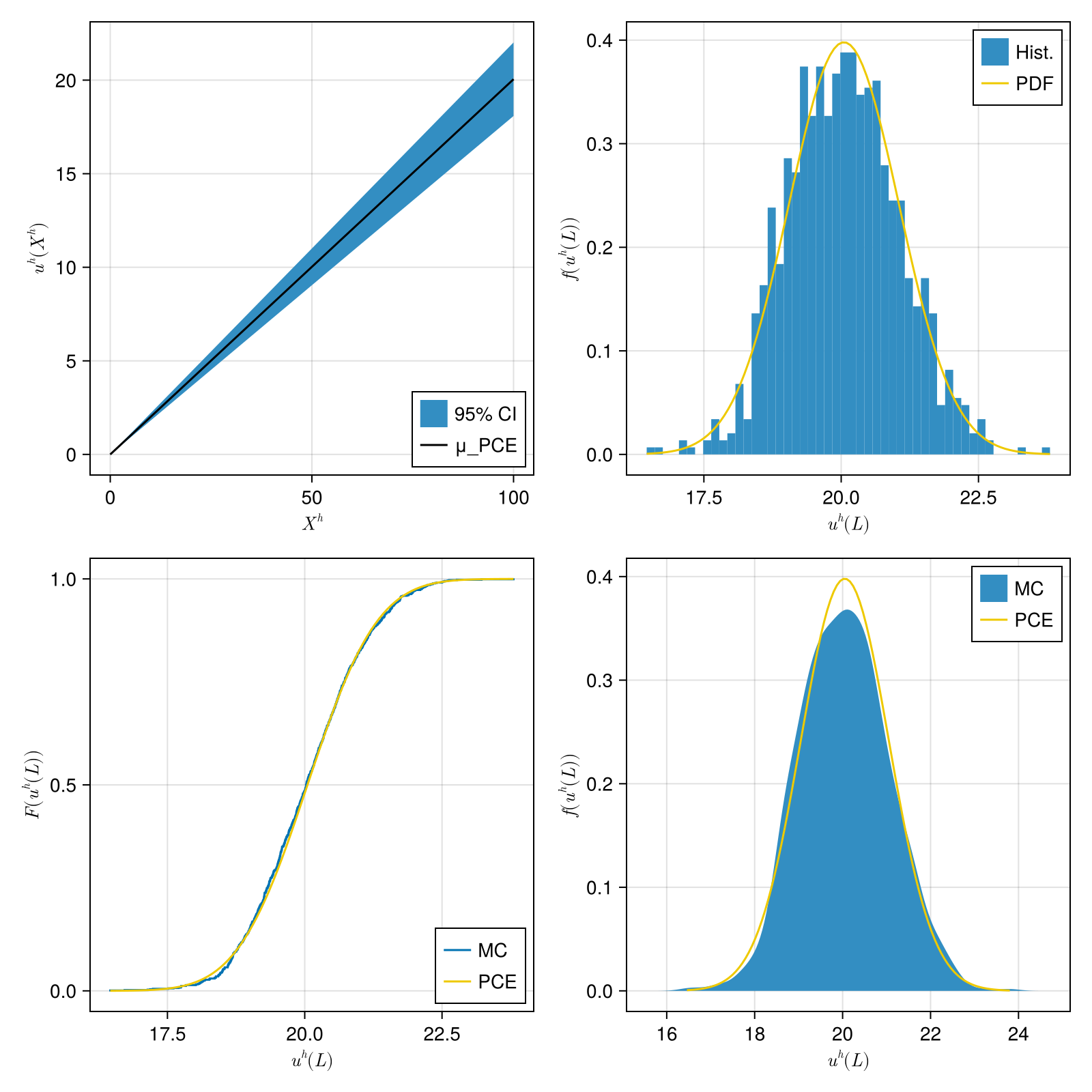
The figures show:

• (a) the mean displacement and 95% confidence interval of the PCE surrogate
• (b) the histogram of the Monte Carlo sample compared to the PDF of the PCE surrogate at $X=100$
• (c) the empirical CDF of the Monte Carlo sample compared to the PCE surrogate at $X=100$
• (d) the empirical PDF of the Monte Carlo sample compared to the PCE surrogate at $X=100$

module Example101_Sampling1DBarUnderTension

using StatFEMEUCLID
using Random
using Distributions
using UMBridge
using CairoMakie

Distributions.LogNormal expects μ and σ of the underlying normal distribution so we need to convert our wanted μ and σ to obtain correct values

function create_lognormal_distribution(μ, σ)
    μ_log = log(μ^2 / sqrt(μ^2 + σ^2))
    σ_log = sqrt(log(1 + σ^2 / (μ^2)))
    return LogNormal(μ_log, σ_log)
end

With server_url you can point to a different UMBridge server implementing the model the default is what is provided by the ExtendableFEM.jl-based implementation here but we also have an implementation based on Kratos here, which listens on http://localhost:4242 by default.

function main(;
        μ_E = 200.0,
        σ_E = 10.0,
        n_MonteCarlo = 1000,
        n_PCE = 50,
        server_url = "http://localhost:4343",
        gridpoint_index = 50,
    )

    rng = MersenneTwister(2020)  #fixed seed for comparability between runs

    fem_model = UMBridge.HTTPModel("Bar1D.FEM", server_url)
    lognormal_dist = create_lognormal_distribution(μ_E, σ_E)

Now we perform sampling of the black box through the Sampling submodule

    sample_MC = StatFEMEUCLID.Sampling.sample_FEM(fem_model, n_MonteCarlo, sample_distribution = lognormal_dist, rng = rng)
    sample_PCE = StatFEMEUCLID.Sampling.sample_FEM(fem_model, n_PCE, sample_distribution = lognormal_dist, rng = rng)

For the Monto Carlo sample we directly compute the empirical standard deviation

    _, σ_MC = StatFEMEUCLID.Sampling.compute_statistics(sample_MC)

With the other (smaller!) sample we use the PCE submodule to create a surrogate and calculate it's mean and standard deviation.

    pce_surrogate = StatFEMEUCLID.PCE.PolyChaosExpansion(sample_PCE)
    μ_PCE, σ_PCE = StatFEMEUCLID.PCE.compute_statistics(pce_surrogate)

    return plot_variations(μ_PCE, σ_PCE, sample_MC, gridpoint_index)
end

This function generates all the plots shown above based on the PCE surrogate and the Monte Carlo sample

function plot_variations(μ_PCE, σ_PCE, sample_MC, gridpoint_index)

    MC_sample_at_gridpoint = sample_MC.fem_sample[:, gridpoint_index]
    f = Figure(size = (800, 800))

Data for the first plot: confidence interval of the bar displacement

    xgrid = LinRange(0, 100, 50)
    confidence_factor_95p = 1.96
    lower_percentile = μ_PCE - confidence_factor_95p * σ_PCE
    upper_percentile = μ_PCE + confidence_factor_95p * σ_PCE

    #Data for the other plots,
    #i.e. related to the displacement at the tip of the bar

    x_L = Vector(LinRange(minimum(MC_sample_at_gridpoint), maximum(MC_sample_at_gridpoint), 100))
    PCE_distribution = Normal(μ_PCE[gridpoint_index], σ_PCE[gridpoint_index])

    #Axes with labels
    ax11 = Axis(f[1, 1], xlabel = L"X^h", ylabel = L"u^h(X^h)")
    ax12 = Axis(f[1, 2], xlabel = L"u^h(L)", ylabel = L"f(u^h(L))")
    ax21 = Axis(f[2, 1], xlabel = L"u^h(L)", ylabel = L"F(u^h(L))")
    ax22 = Axis(f[2, 2], xlabel = L"u^h(L)", ylabel = L"f(u^h(L))")

    band!(f[1, 1], xgrid, lower_percentile, upper_percentile; label = "95% CI")
    lines!(f[1, 1], xgrid, μ_PCE; color = :black, label = "μ_PCE")

    hist!(f[1, 2], MC_sample_at_gridpoint, bins = 50, normalization = :pdf; label = "Hist.")
    lines!(f[1, 2], x_L, pdf.(PCE_distribution, x_L), color = :gold2; label = "PDF")

    ecdfplot!(f[2, 1], MC_sample_at_gridpoint; label = "MC")
    lines!(f[2, 1], x_L, cdf.(PCE_distribution, x_L), color = :gold2; label = "PCE")

    density!(f[2, 2], MC_sample_at_gridpoint; label = "MC")
    lines!(f[2, 2], x_L, pdf.(PCE_distribution, x_L), color = :gold2; label = "PCE")

    axislegend(ax11, position = :rb)
    axislegend(ax12, position = :rt)
    axislegend(ax21, position = :rb)
    axislegend(ax22, position = :rt)
    return f
end

end

This page was generated using Literate.jl.