203: Model parameter identification for a 2D Plate with a hole based on sparse and noisy data

(source code)

In this example we combine the two previous examples, i.e. the data assimilation from 201 with the model parameter identification of example 202. The goal is to re-identify a known truth that was used to generate synthetic data. The main difference to 202 is that the synthetic data is only measured at a few distinct sensor locations and that additional measurement noise is applied to it.

A single loop of the full algorithm works as follows;

given a current guess $\kappa^t$ sample and compute a PCE surrogate $u_f^t$
if $\text{RMSE}(u_f^t,y) < TOL$ we have found a suitable model $\kappa^*=\kappa^t$, finish
if not, assimilate posterior state $u_a^t$ using StatFEM
Identify model parameters $\kappa^{t+1}$ based on $u_a^t$ (calibration or discovery)
If maximum number of iterations is reached, abort. Else, redo loop with $\kappa^{t+1}$.

As before we have two options for identifying the model

StatFEM-VFM-EGM, using calibration internally
StatFEM-EUCLID, using discovery internally

The following figure shows the 38 sensor locations on the mesh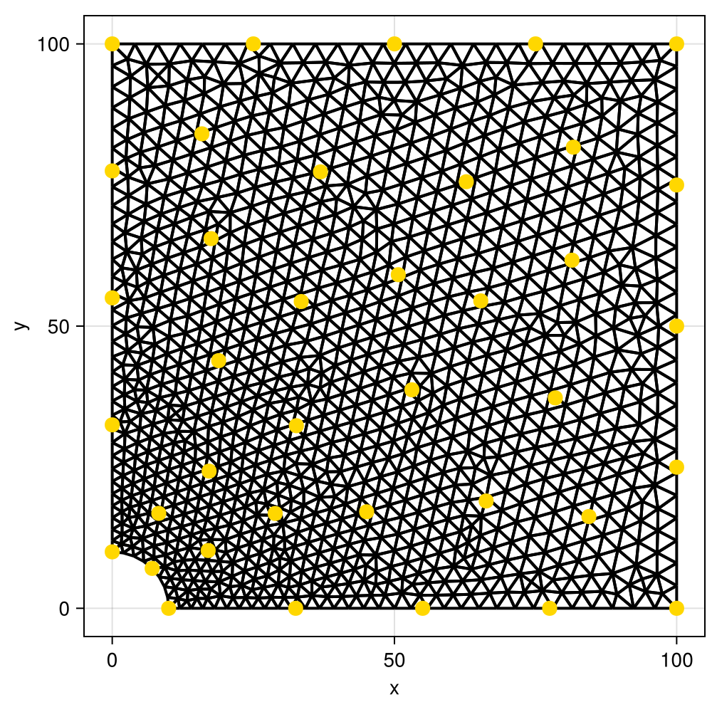

Results

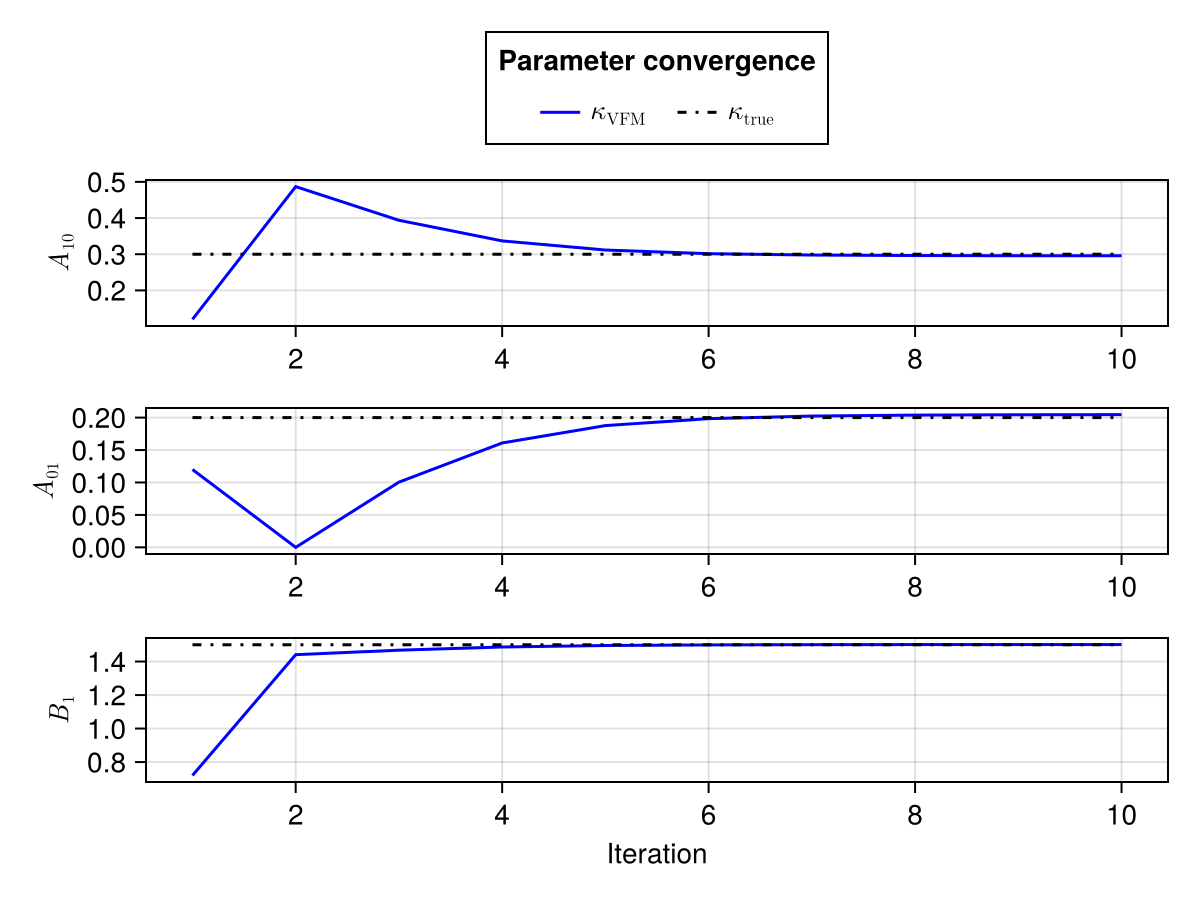
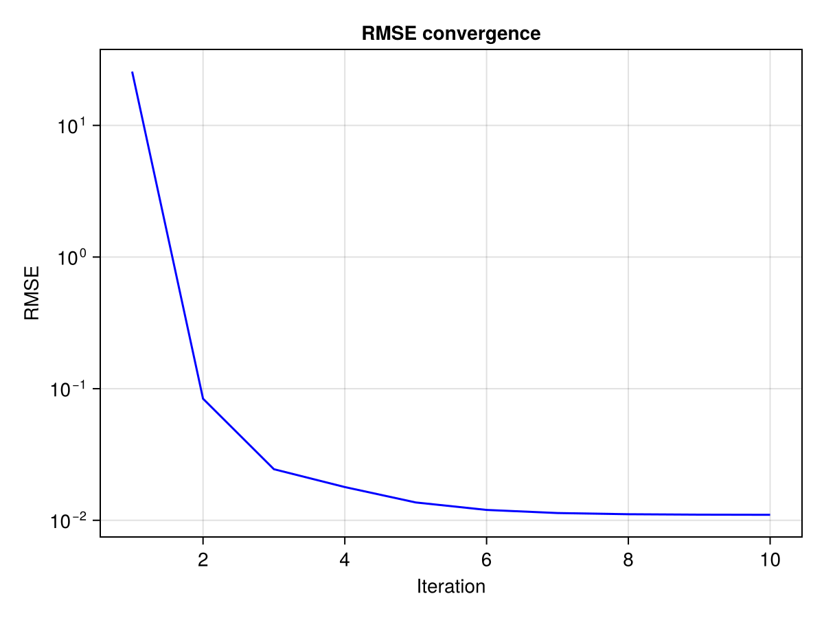
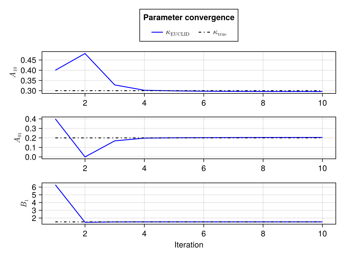
For both algorithms we want to look at the convergence of the three nonzero parameters to the true values as well as the convergence of the RMSE between the

StatFEM-VFM-EGM

StatFEM-EUCLID

Important

Remember to start your UMBridge FEM server before running the example!

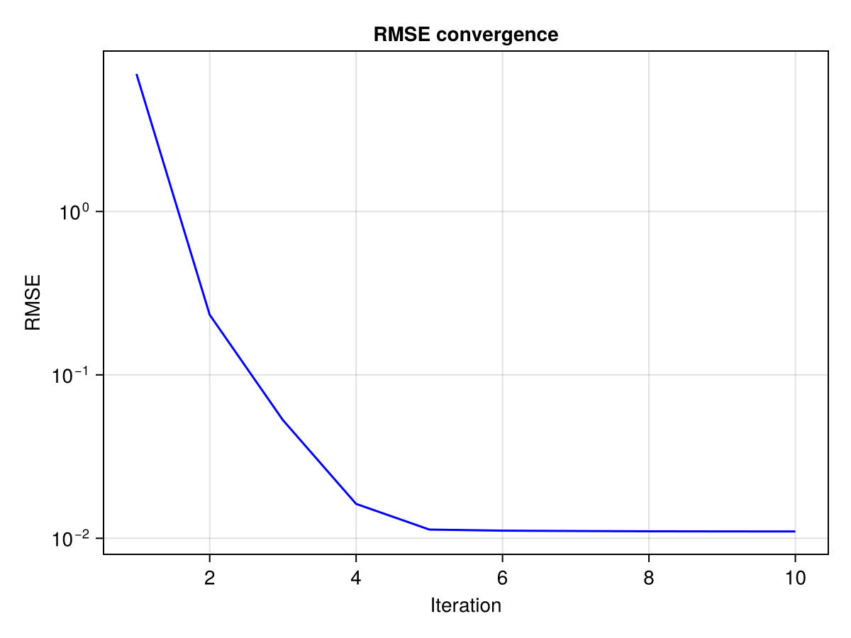
module Example203_StaFEM_EUCLID_PlateWithHole

using StatFEMEUCLID
using Random
using Distributions
using CairoMakie
using Gmsh
using PolyChaos
using ExtendableGrids
using GridVisualize
using CSV, DataFrames
using Optim
using UMBridge
using LineSearches
using LinearAlgebra

With server_url you can point to a different UMBridge server implementing the model the default is what is provided by the Ferrite.jl-based implementation here

function main(;
        μ_F = 0.5,
        σ_F = 2.5e-2,
        n_PCE = 30,
        E = 2.7,
        ν = 0.35,
        σ_sensor = 0.001,
        server_url = "http://localhost:4232"
    )
    rng = MersenneTwister(2530)  #fixed seed for comparability between runs

As before we define our UMBrige models

    model_name = "HolePlate2D"
    fem_model = UMBridge.HTTPModel(model_name * ".FEM", server_url)
    residual_model = UMBridge.HTTPModel(model_name * ".residual", server_url)
    projection_model = UMBridge.HTTPModel(model_name * ".projection", server_url)

Read in the sensors, grid and (synthetic) measurements

    sensor_set = CSV.read("Example203_sensors.csv", EqualSensorSet{Float64}, σ_sensor)
    n_dofs = UMBridge.model_output_sizes(fem_model)[1]
    calculate_projection_matrix(sensor_set, projection_model, n_dofs)

    grid = ExtendableGrids.simplexgrid_from_gmsh("Example201_mesh.msh", Tc = Float64, Ti = Int64)

    dataframe_measurements = CSV.read("Example203_measurements.csv", DataFrame)
    measurements = [Vector{Float64}(row) for row in eachrow(dataframe_measurements)]
    n_sen = length(measurements)

Measurements are stored as ux, uy so we need to reorder them to be a single vector

    u_measurements = zeros(2 * n_sen)
    for i in eachindex(measurements)
        u_measurements[i] = measurements[i][1]
        u_measurements[n_sen + i] = measurements[i][2]
    end

Setup for StatFEM_VFM_EGM and StatFEM_EUCLID is practically identical

Define κtrue for plotting and κ0 as initial guess

    κ_true_vfm = [0.3, 0.2, 1.5]
    κ_0_vfm_egm = [0.12, 0.12, 0.72]

Combine HTTPModel information in InverseModelConfig struct VFM-EGM uses calibration, so the known model with nMR=1 and nVOL=1

    vfm_egm_config = InverseModelConfig(
        fem_model, residual_model,
        Dict{String, Any}(
            "material" => "MooneyRivlin",
            "n_MR" => 1,
            "n_VOL" => 1
        ),
        μ_F
    )

Run StatFEMVFMEGM as defined below

    i_ve, κ_history_ve, rmse_history_ve = StatFEM_VFM_EGM(
        vfm_egm_config, κ_0_vfm_egm, sensor_set, u_measurements,
        rng = rng, sample_distribution = Normal(μ_F, σ_F)
    )

Define κtrue for plotting and κ0 as initial guess

    κ_true_euclid = [0.3, 0.2, 0.0, 0.0, 0.0, 0.0, 0.0, 0.0, 0.0, 1.5]
    κ_0_euclid = [0.4, 0.4, 0.3, 0.3, 0.3, 0.1, 0.1, 0.1, 0.1, 6.3]

Combine HTTPModel information in InverseModelConfig struct VFM-EGM uses discovery, so the larger model with nMR=3 and nVOL=1

    euclid_config = InverseModelConfig(
        fem_model, residual_model,
        Dict{String, Any}(
            "material" => "MooneyRivlin",
            "n_MR" => 3,
            "n_VOL" => 1
        ),
        μ_F
    )

Run StatFEM_EUCLID as defined below

    i_euclid, κ_history_euclid, rmse_history_euclid = StatFEM_EUCLID(
        euclid_config, κ_0_euclid, sensor_set, u_measurements,
        rng = rng, sample_distribution = Normal(μ_F, σ_F)
    )

Generate all the plots that we want to return

    fig_vfm_param = plot_vfm_parameters(i_ve, κ_history_ve, κ_true_vfm)
    fig_vfm_rmse = plot_rmse(i_ve, rmse_history_ve)
    fig_euclid_param = plot_euclid_parameters(i_euclid, κ_history_euclid, κ_true_euclid)
    fig_euclid_rmse = plot_rmse(i_euclid, rmse_history_euclid)
    sensorvis = plot_sensors(grid, sensor_set.locations)

    return fig_vfm_param, fig_vfm_rmse, fig_euclid_param, fig_euclid_rmse, sensorvis
end

As in Example202 we want to penalize the larger model to get a compressible material

function MooneyRivlin_penalization(penalty_multiplier, penalization_weight)
    function f(κ)
        return abs(sum(κ[1:(end - 1)]) * penalty_multiplier - κ[end]) * penalization_weight
    end
    function g!(G, κ)
        s = sign(sum(κ[1:(end - 1)] * penalty_multiplier) - κ[end])
        G[1:(end - 1)] .+= penalization_weight * penalty_multiplier * s
        return G[end] -= penalization_weight * s
    end

    return f, g!
end

function StatFEM_VFM_EGM(
        config::InverseModelConfig, κ_0, sensor_set, u_measurements;
        optimizer = Fminbox(BFGS(linesearch = BackTracking())),
        optimizer_options = Optim.Options(), maxiter = 10, n_PCE = 50, rng = default_rng(), sample_distribution = Normal(0.0, 1.0), TOL = 1.0e-4
    )

    @info "StatFEM_VFM_EGM"

    #allocate intermediate and result vectors
    κ_history = zeros(maxiter, length(κ_0))
    rmse_history = zeros(maxiter)
    κ_t = deepcopy(κ_0)
    n_dofs = UMBridge.model_output_sizes(config.fem_model)[1]
    n_sen = size(sensor_set)
    u_a = zeros(2 * n_dofs)


    lower = zeros(length(κ_t))
    upper = 10.0 * ones(length(κ_t))

    i = 1
    while (true)
        @info "Starting iteration $i"

As described above we start by sampling and constructing a PCE surrogate (Example101)

        prior_sample = sample_FEM(
            config.fem_model,
            n_PCE,
            sample_distribution = sample_distribution,
            rng = rng,
            config = config.config,
            extra_params = κ_t,
            solution_index = :
        )

        pce_surrogate = PolyChaosExpansion(prior_sample, polynomials = GaussOrthoPoly(4))
        μ_u_f = mean(pce_surrogate)

Check if the mean displacements of the surrogate are close enough to the measurements

        κ_history[i, :] = κ_t
        rmse_history[i] = model_rmse(μ_u_f, sensor_set, u_measurements)
        @info rmse_history[i]
        if (rmse_history[i] < TOL)
            @info "Found sufficient model with RMSE=" rmse_history[i]
            return i, κ_history, rmse_history
        end

or if maxiter was reached

        if i == maxiter
            @info "Reached maximum number of iterations, aborting"
            return i, κ_history, rmse_history
        end

Take the ux and uy subviews of the PCE to calculate the StatFEM posterior (Example 201)

        pce_surrogate_x = PolyChaosExpansion(pce_surrogate.coefficients[:, 1:n_dofs], pce_surrogate.orthogonal_polynomials)
        pce_surrogate_y = PolyChaosExpansion(pce_surrogate.coefficients[:, (n_dofs + 1):(2 * n_dofs)], pce_surrogate.orthogonal_polynomials)

        u_a[1:n_dofs] = posterior_mean(sensor_set, u_measurements[1:n_sen], pce_surrogate_x)
        u_a[(n_dofs + 1):(2 * n_dofs)] = posterior_mean(sensor_set, u_measurements[(n_sen + 1):(2 * n_sen)], pce_surrogate_y)

As in Example 202 compute next κ_t through calibration

        f_cal, g_cal! = create_residual_objective_and_gradient(config.residual_model, u_a; config = config.config)
        optimal_residual = optimize(f_cal, g_cal!, lower, upper, κ_t, optimizer, optimizer_options)
        κ_t = Optim.minimizer(optimal_residual)

        @show κ_t
        i += 1
    end
    return
end


function StatFEM_EUCLID(config::InverseModelConfig, κ_0, sensor_set, u_measurements; optimizer = Fminbox(BFGS(linesearch = BackTracking())), optimizer_options = Optim.Options(time_limit = 200), maxiter = 10, n_PCE = 50, rng = default_rng(), sample_distribution = Normal(0.0, 1.0), TOL = 1.0e-4)
    @info "StatFEM_EUCLID"

    κ_history = zeros(maxiter, length(κ_0))
    rmse_history = zeros(maxiter)
    κ_t = deepcopy(κ_0)
    n_dofs = UMBridge.model_output_sizes(config.fem_model)[1]
    n_sen = size(sensor_set)
    u_a = zeros(2 * n_dofs)

    lower = zeros(length(κ_t))
    upper = 10.0 * ones(length(κ_t))

For EUCLID we also need to define the lasso sweep and get the penalty function and gradient

    lasso_sweep = 5 * logrange(1.0e-5, 1.0, 6)
    f_mr_penalty, g_mr_penalty! = MooneyRivlin_penalization(3.0, 10.0)

    i = 1

Apart from the model identification the loop is identical to the one in StatFEMVFMEGM

    while (true)
        @info "Starting iteration $i"
        prior_sample = sample_FEM(
            config.fem_model,
            n_PCE,
            sample_distribution = sample_distribution,
            rng = rng,
            config = config.config,
            extra_params = κ_t,
            solution_index = :
        )

Sample and construct PCE surrogate

        pce_surrogate = PolyChaosExpansion(prior_sample, polynomials = GaussOrthoPoly(4))
        μ_u_f = mean(pce_surrogate)

Check if the mean displacements of the surrogate are close enough to the measurements

        κ_history[i, :] = κ_t
        rmse_history[i] = model_rmse(μ_u_f, sensor_set, u_measurements)
        @info rmse_history[i]
        if (rmse_history[i] < TOL)
            @info "Found sufficient model with RMSE=" rmse_history[i]
            return i, κ_history, rmse_history
        end

or if maxiter was reached

        if i == maxiter
            @info "Reached maximum number of iterations, aborting"
            return i, κ_history, rmse_history
        end

Take the ux and uy subviews of the PCE to calculate the StatFEM posterior (Example 201)

        pce_surrogate_x = PolyChaosExpansion(pce_surrogate.coefficients[:, 1:n_dofs], pce_surrogate.orthogonal_polynomials)
        pce_surrogate_y = PolyChaosExpansion(pce_surrogate.coefficients[:, (n_dofs + 1):(2 * n_dofs)], pce_surrogate.orthogonal_polynomials)

        u_a[1:n_dofs] = posterior_mean(sensor_set, u_measurements[1:n_sen], pce_surrogate_x)
        u_a[(n_dofs + 1):(2 * n_dofs)] = posterior_mean(sensor_set, u_measurements[(n_sen + 1):(2 * n_sen)], pce_surrogate_y)

As in example 202 compute next κ_t through discovery/EUCLID

        κ_t, _ = EUCLID(
            config, lasso_sweep, κ_t, sensor_set, u_a, u_measurements,
            f_penalty = f_mr_penalty, g_penalty = g_mr_penalty!,
            upper = upper, lower = lower,
            show_info = false, use_gradient = true,
            optimizer = optimizer,
            optimizer_options = optimizer_options
        )

        @show κ_t
        i += 1
    end
    return
end

function plot_vfm_parameters(i, κ_history, κ_true)
    fig = Figure()

    ax_A10 = Axis(fig[1, 1], ylabel = L"A_{10}")
    ax_A01 = Axis(fig[2, 1], ylabel = L"A_{01}")
    ax_B1 = Axis(fig[3, 1], ylabel = L"B_1", xlabel = "Iteration")

    lines!(ax_A10, 1:i, κ_history[1:i, 1], color = :blue, label = L"\kappa_\text{VFM}")
    lines!(ax_A01, 1:i, κ_history[1:i, 2], color = :blue)
    lines!(ax_B1, 1:i, κ_history[1:i, 3], color = :blue)
    lines!(ax_A10, [1, i], [κ_true[1], κ_true[1]], color = :black, linestyle = :dashdot, label = L"\kappa_\text{true}")
    lines!(ax_A01, [1, i], [κ_true[2], κ_true[2]], color = :black, linestyle = :dashdot)
    lines!(ax_B1, [1, i], [κ_true[3], κ_true[3]], color = :black, linestyle = :dashdot)


    fig[0, :] = Legend(fig, ax_A10, "Parameter convergence", orientation = :horizontal)


    return fig
end

function plot_euclid_parameters(i, κ_history, κ_true)
    fig = Figure()

    ax_A10 = Axis(fig[1, 1], ylabel = L"A_{10}")
    ax_A01 = Axis(fig[2, 1], ylabel = L"A_{01}")
    ax_B1 = Axis(fig[3, 1], ylabel = L"B_1", xlabel = "Iteration")

    lines!(ax_A10, 1:i, κ_history[1:i, 1], color = :blue, label = L"\kappa_\text{EUCLID}")
    lines!(ax_A01, 1:i, κ_history[1:i, 2], color = :blue)
    lines!(ax_B1, 1:i, κ_history[1:i, 10], color = :blue)
    lines!(ax_A10, [1, i], [κ_true[1], κ_true[1]], color = :black, linestyle = :dashdot, label = L"\kappa_\text{true}")
    lines!(ax_A01, [1, i], [κ_true[2], κ_true[2]], color = :black, linestyle = :dashdot)
    lines!(ax_B1, [1, i], [κ_true[10], κ_true[10]], color = :black, linestyle = :dashdot)


    fig[0, :] = Legend(fig, ax_A10, "Parameter convergence", orientation = :horizontal)


    return fig
end

function plot_rmse(i, rmse_history)
    fig = Figure()

    ax = Axis(fig[1, 1], yscale = log10, ylabel = "RMSE", xlabel = "Iteration", title = "RMSE convergence")

    lines!(ax, 1:i, rmse_history[1:i], color = :blue)


    return fig
end

This function generates the synthetic data based on a Mooney-Rivlin model. Note that the forward model has to be able to solve with this material model to regenerate the data. The data in the repository has been generated using the default, i.e. the Ferrite.jl-based implementation here

function generate_synthetic_data(;
        F = 0.5,
        σ_sensor = 0.001,
        server_url = "http://localhost:4232"
    )

Note that we also need the projection model here since we want to map the FEM solution to the given sensor points.

    model_name = "HolePlate2D"
    fem_model = UMBridge.HTTPModel(model_name * ".FEM", server_url)
    projection_model = UMBridge.HTTPModel(model_name * ".projection", server_url)

    A_10 = 0.3
    A_01 = 0.2
    B_1 = 1.5

    κ = [A_10, A_01, B_1]

We want to solve with the smallest Mooney-Rivlin model with a total of three parameters

    MR_material_config = Dict{String, Any}(
        "material" => "MooneyRivlin",
        "n_MR" => 1,
        "n_VOL" => 1
    )
    n_dofs = UMBridge.model_output_sizes(fem_model)[1]

Since we solve with the exact mean traction force, we don't have to sample and can directly evaluate the forward model once.

    u_truth = evaluate_fem_model(
        fem_model, F, solution_index = :, config = MR_material_config, extra_params = κ
    )

Then, we read in the sensor locations and obtain the projection matrix

    sensor_set = CSV.read("Example203_sensors.csv", EqualSensorSet{Float64}, σ_sensor)
    n_sen = size(sensor_set)
    calculate_projection_matrix(sensor_set, projection_model, n_dofs)

and project the solution onto the sensor points

    u_measured = project(sensor_set, u_truth)

Finally, we apply a Gaussian noise to the projected measurements

    apply_noise!(sensor_set, reshape(u_measured, (n_sen, 2)); rng = MersenneTwister(2530))

before writing the result to file.

    dataframe_measurements = DataFrame(u_x = u_measured[1:n_sen], u_y = u_measured[(n_sen + 1):(2 * n_sen)])
    return CSV.write("Example203_measurements.csv", dataframe_measurements)
end

Plot the underlying grid as well as the sensor points

function plot_sensors(grid, sensor_points::Vector{Vector{Float64}})

    sensorvis = GridVisualizer(; Plotter = CairoMakie)

    gridplot!(sensorvis, grid, show_colorbar = false)
    x = zeros(length(sensor_points))
    y = zeros(length(sensor_points))
    for i in eachindex(sensor_points)
        x[i] = sensor_points[i][1]
        y[i] = sensor_points[i][2]
    end
    customplot!(sensorvis) do ax
        CairoMakie.scatter!(ax, x, y, color = :gold, markersize = 15)
    end
    return sensorvis
end

#The following functions override the default behaviour of GridVisualizeTools
#to remove coloring of cells and boundaries from the sensor plot.
using Colors
import GridVisualizeTools: region_cmap, bregion_cmap
function region_cmap(n)
    return fill(RGB(1.0, 1.0, 1.0), n)
end

function bregion_cmap(n)
    return fill(RGBA(0.0, 0.0, 0.0, 0.0), n)
end

end

This page was generated using Literate.jl.